- / -

EMSC3025/6025: Remote Sensing of Water Resources

Dr. Sia Ghelichkhan

- / -

Groundwater — Principles

EMSC3025/6025

Dr. Sia Ghelichkhan

Objectives

By the end of this lecture, you should be able to:

Understand the theory of saturated groundwater flow.
Derive and apply the basic groundwater flow equation.
Use flow nets to estimate hydraulic head distribution and flow paths.
Identify boundary and initial conditions for analytical solutions.
Solve simple steady-state flow problems using analytical methods.

A refresher on some basic math

Understanding Differential Equations in Groundwater

Many students find the quantitative aspects of groundwater hydrology challenging at first glance. 😱

A differential equation like this immediately suggests advanced mathematical concepts:

\frac{\partial}{\partial x} \left( T_x \frac{\partial h}{\partial x} \right) + \frac{\partial}{\partial y} \left( T_y \frac{\partial h}{\partial y} \right) + \frac{\partial}{\partial z} \left( T_z \frac{\partial h}{\partial z} \right) = S \frac{\partial h}{\partial t}

Good news: At this introductory level, we don’t need to solve these equations—just recognise and understand them.

Key Point

Hydrogeology provides simplified approaches for dealing with these equations.

Recognising Equation Features

You don’t need to be a math person for dealing with groundwater equations.Even as toddlers, we could recognise a rhinoceros by its features:

Four stubby legs
Two horns on an ugly-looking head

Similarly, differential equations have recognizable features that tell us what we’re dealing with.

The unknown we’re trying to find is usually hidden in derivative terms like:

\frac{\partial h}{\partial x} \text{ or } \frac{\partial h}{\partial y} \text{ or } \frac{\partial h}{\partial z}

where h is our unknown (hydraulic head).

What Makes an Equation What It Is?

The unknown variable determines the equation type:

h (hydraulic head) → groundwater flow equation
C (concentration) → mass transport equation
T (temperature) → energy transport equation

The “stuff” on the right-hand side are functions of time and space variables (t, x, y, z) and various parameters.

Determining Problem Characteristics

Step 1: Identify the unknown

What variable are we solving for?

Step 2: Count space dimensions

How many spatial directions does flow occur in?

Step 3: Check for time dependence

Does the solution change with time?

Example Analysis:

\frac{\partial^2 h}{\partial x^2} = 0

Unknown: h → groundwater flow
Dimensions: Only x → 1D problem
Time: No \frac{\partial h}{\partial t} → steady-state
Parameters: None → simple case

Problem Dimensionality

Dimensionality describes how many directions the unknown (hydraulic head) changes.

1D: Head changes in one direction only
2D: Head changes in two directions
3D: Head changes in three directions

Important: This refers to how many spatial variables appear in the equation, not the physical geometry.

Example

A 3D aquifer between two rivers might still have 1D flow if water only moves in the x-direction.

Steady-State vs. Transient

Steady-State:

No time term: \frac{\partial h}{\partial t} = 0
Hydraulic head doesn’t change with time
Easier to solve

Transient:

Time term present: \frac{\partial h}{\partial t} \neq 0
Hydraulic head changes with time
More complex solutions

Practice Question

Look at your flow equation. Is there a \frac{\partial h}{\partial t} term?

Yes → Transient problem
No → Steady-state problem

Parameter Dependencies

Sometimes equations contain parameters like K, T, or S.

If parameters are constant everywhere → hydraulic head distribution is independent of parameter values
If parameters vary in space → hydraulic head depends on parameter values

Practical impact: You can solve for the pattern of flow, then scale it based on actual parameter values.

Differential Equations of Groundwater Flow

What sets hydrogeology apart is its emphasis on mathematical treatment of physical processes.

The goal: determine how hydraulic head varies throughout a domain.

Three Essential Components:

Governing equation – describes groundwater flow
Domain – geometry and layering
Boundary conditions – head or flux at boundaries

Figure 5.1 — From physical system to solution: geometry → equation → head → flow pattern

What Do We Get From Solving the Equation?

Once we solve for the hydraulic head distribution, we can:

Draw equipotentials (contours of equal head)
Deduce flow paths (direction of groundwater movement)
Calculate flow rates between different points
Predict impacts of pumping or recharge

Flow Domain vs. Flow Equation Dimensionality

Important Distinction:

The dimensionality of the flow domain ≠ dimensionality of the flow equation

A 1D equation can describe flow in a 3D domain if flow occurs in one direction only
The actual direction of water movement determines equation dimensionality

River-aquifer system — Flow is 1D even in a 3D system

Example: 1D Flow in 3D Domain

Case Study: Aquifer Between Two Rivers

Physical structure: 3D confined aquifer
Flow direction: Only in x-direction (river to river)
Governing equation: 1D flow equation
Why? No head variation in y or z directions

\frac{\partial}{\partial x} \left( T_x \frac{\partial h}{\partial x} \right) = S \frac{\partial h}{\partial t}

Key Insight:

Look at the flow pattern, not the aquifer geometry, to determine equation dimensionality.

Deriving Groundwater Flow Equations

Starting Point: Conservation of Mass

Groundwater flow equations come from mass conservation applied to a representative elementary volume (REV).

Think of a small cube of aquifer material — water flows in and out through all six faces.

REV and flow directions — Control volume to derive the equation

The Conservation Principle

\text{mass inflow} - \text{mass outflow} = \text{change in storage over time}

What we account for:

Flow through all six faces of the REV
Water density (\rho_w)
Porosity (n)
Velocity components in x, y, z directions

Physical meaning:

If more water flows in than out → head rises
If more water flows out than in → head drops
If inflow = outflow → steady-state

Mathematical Representation of Conservation

M_{x1} - M_{x2} + M_{y1} - M_{y2} + M_{z1} - M_{z2} = \frac{\partial}{\partial t} (\rho_w n \Delta x \Delta y \Delta z)

Breaking down the equation:

M_{x1}, M_{x2} = mass flow in x-direction (in and out)
M_{y1}, M_{y2} = mass flow in y-direction (in and out)
M_{z1}, M_{z2} = mass flow in z-direction (in and out)
Right side = rate of mass accumulation in the REV

Translation: Net mass inflow = rate of mass accumulation

Mass Flux Derivation: Step-by-Step

X-Direction Flow

Consider flow entering and leaving the REV in the x-direction:

Inflow at left face:

M_{x1} = \left[ \rho_w q_x - \frac{1}{2} \frac{\partial (\rho_w q_x)}{\partial x} \Delta x \right] \Delta y \Delta z

Outflow at right face:

M_{x2} = \left[ \rho_w q_x + \frac{1}{2} \frac{\partial (\rho_w q_x)}{\partial x} \Delta x \right] \Delta y \Delta z

Key Concept:

Flow varies across the REV due to spatial gradients. We use Taylor expansion around the center point.

Net Flow in X-Direction

Net x-direction inflow: M_{x1} - M_{x2} = - \frac{\partial (\rho_w q_x)}{\partial x} \Delta x \Delta y \Delta z

Same logic applies to y and

M_{y1} - M_{y2} = - \frac{\partial (\rho_w q_y)}{\partial y} \Delta x \Delta y \Delta z

and to z direction:

M_{z1} - M_{z2} = - \frac{\partial (\rho_w q_z)}{\partial z} \Delta x \Delta y \Delta z

Combining All Directions: Full Conservation

- \left[ \frac{\partial (\rho_w q_x)}{\partial x} + \frac{\partial (\rho_w q_y)}{\partial y} + \frac{\partial (\rho_w q_z)}{\partial z} \right] = \frac{\partial (\rho_w n)}{\partial t}

This equation combines:

Net inflow from all three directions (left side)
Rate of mass accumulation (right side)

Next step: Simplify by assuming water density is constant

Physical meaning:

Divergence of flow = storage change

Assuming Constant Water Density

- \left[ \frac{\partial q_x}{\partial x} + \frac{\partial q_y}{\partial y} + \frac{\partial q_z}{\partial z} \right] = \frac{1}{\rho_w} \frac{\partial (\rho_w n)}{\partial t}

Why this assumption? For most groundwater problems, water density changes are negligible compared to flow effects.

Introducing Specific Storage

The right-hand side can be simplified using specific storage (S_s):

\frac{1}{\rho_w} \frac{\partial (\rho_w n)}{\partial t} = S_s \frac{\partial h}{\partial t}

Definition: S_s accounts for water release due to both aquifer compression and water expansion.

Remember:

S_s links changes in storage to changes in hydraulic head.

Conservation in Terms of Hydraulic Head

\frac{\partial q_x}{\partial x} + \frac{\partial q_y}{\partial y} + \frac{\partial q_z}{\partial z} = - S_s \frac{\partial h}{\partial t}

We’re almost there! Next step: substitute Darcy’s law to express everything in terms of hydraulic head.

Applying Darcy’s Law

Darcy’s Law in 3D:

q_x = -K_x \frac{\partial h}{\partial x}
q_y = -K_y \frac{\partial h}{\partial y}
q_z = -K_z \frac{\partial h}{\partial z}

Substituting into our conservation equation…

Key insight:

Darcy’s law relates flow to head gradients using hydraulic conductivity.

The Final Groundwater Flow Equation

\frac{\partial}{\partial x} \left( K_x \frac{\partial h}{\partial x} \right) + \frac{\partial}{\partial y} \left( K_y \frac{\partial h}{\partial y} \right) + \frac{\partial}{\partial z} \left( K_z \frac{\partial h}{\partial z} \right) = S_s \frac{\partial h}{\partial t}

This is the fundamental equation for flow in saturated porous media!

What it describes:

How hydraulic head (h) varies in space and time
3D flow in heterogeneous, anisotropic media

Parameters needed:

K_x, K_y, K_z = hydraulic conductivity
S_s = specific storage
Boundary and initial conditions

Special Case 1: Steady-State Flow

When \frac{\partial h}{\partial t} = 0 (no change in head with time):

Physical meaning:

System has reached equilibrium
Inflow = outflow everywhere
Head pattern is time-invariant
Much easier to solve than transient problems

Example situations:

Long-term pumping
Seasonal averages
Regional flow systems

Special Case 2: Isotropic, Homogeneous Media

When K_x = K_y = K_z = K (constant) and steady-state:

\frac{\partial^2 h}{\partial x^2} + \frac{\partial^2 h}{\partial y^2} + \frac{\partial^2 h}{\partial z^2} = 0

This is Laplace’s equation!

Classic partial differential equation
Many analytical solutions available
Foundation for flow net analysis
Widely used in mathematical physics

Simplification:

When properties are uniform, the equation becomes much simpler to solve.

Working with Transmissivity

For confined aquifers, we often use transmissivity:

T_x = K_x \times b (transmissivity in x-direction)
S = S_s \times b (storativity)
b = aquifer thickness

\frac{\partial}{\partial x} \left( T_x \frac{\partial h}{\partial x} \right) + \frac{\partial}{\partial y} \left( T_y \frac{\partial h}{\partial y} \right) = S \frac{\partial h}{\partial t}

Why transmissivity?

For confined aquifers, flow is integrated over the thickness, making T more practical.

Including Sources and Sinks

Real systems have sources and sinks:

Wells (pumping or injection)
Recharge from precipitation
Leakage to/from other layers

Adding source term Q(x,y,z,t):

Sign convention:

Q > 0 = source (injection)
Q < 0 = sink (pumping)

Special Case 3: Unconfined Aquifers

Dupuit’s Assumption

For unconfined aquifers, we make a simplifying assumption:

Dupuit approximation: Vertical flow is negligible compared to horizontal flow.

Streamlines are horizontal
Hydraulic gradient equals water table slope
Valid when horizontal distances >> aquifer thickness

Dupuit flow — a) actual flow, b) Dupuit approximation

Boussinesq’s Equation

Under Dupuit approximation:

\frac{\partial}{\partial x} \left( K(x,y) h \frac{\partial h}{\partial x} \right) + \frac{\partial}{\partial y} \left( K(x,y) h \frac{\partial h}{\partial y} \right) = S_y \frac{\partial h}{\partial t}

Key features:

h appears both inside and outside derivatives
S_y = specific yield (not specific storage)
Commonly used for water table aquifers

Note:

This is Boussinesq’s equation - the standard for unconfined flow analysis.

Solving the Groundwater Flow Equation

The Missing Piece: Boundary Conditions

The flow equation alone is not enough!

To get a unique solution, we must specify boundary conditions - they define how our domain interacts with the surroundings.

Three main types:

Dirichlet - specify head values
Neumann - specify flow rates
Cauchy - relate head and flow

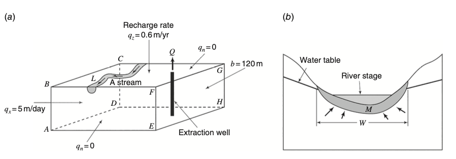Boundary examples Examples of different boundary condition types

Why Boundary Conditions Matter

Without boundary conditions:

Infinite number of possible solutions
No way to determine actual head values
Cannot predict real system behavior

With proper boundary conditions:

Unique solution exists
Realistic head distribution
Meaningful flow predictions

Key applications:

Rivers and lakes (known water levels)
Recharge zones (known flux)
Wells (extraction rates)
No-flow boundaries (impermeable layers)

“Specified Head” Boundaries

In math we call this Dirichlet Boundary Conditions

What it specifies: Hydraulic head values directly

h(x, y, z)|_\text{At a boundary} = h_1(x, y, z, t)

Common examples:

Large lakes or rivers
Ocean boundaries
Artificial ponds or reservoirs

For all of these you can calculate the pressure.

When to use:

When you know the water level at a boundary and it’s much larger than your study area.

Type 2: Neumann Boundary Conditions

“Specified Flux” Boundaries

What it specifies: Water flux (flow rate) across the boundary

q_n|_\text{At a boundary} = q_n(x, y, z, t)

Common examples:

Precipitation recharge (q_n > 0)
Pumping wells (q_n < 0)
Impermeable boundaries (q_n = 0)

Remeber \nabla h \cdot n = q_n

Special case:

q_n = 0 (no-flow) is very common for impermeable rock or clay layers.

Understanding Flux Units

Flux can be expressed two ways:

Darcy velocity q_n [L/T]
- Flow per unit area
- This is the source term we use the flow equation

Volumetric flow rate Q_n [$ L^3/T $]
- Total volume per time
- Used for wells and boundaries

Relationship:

Q_n = q_n \times \text{Area}

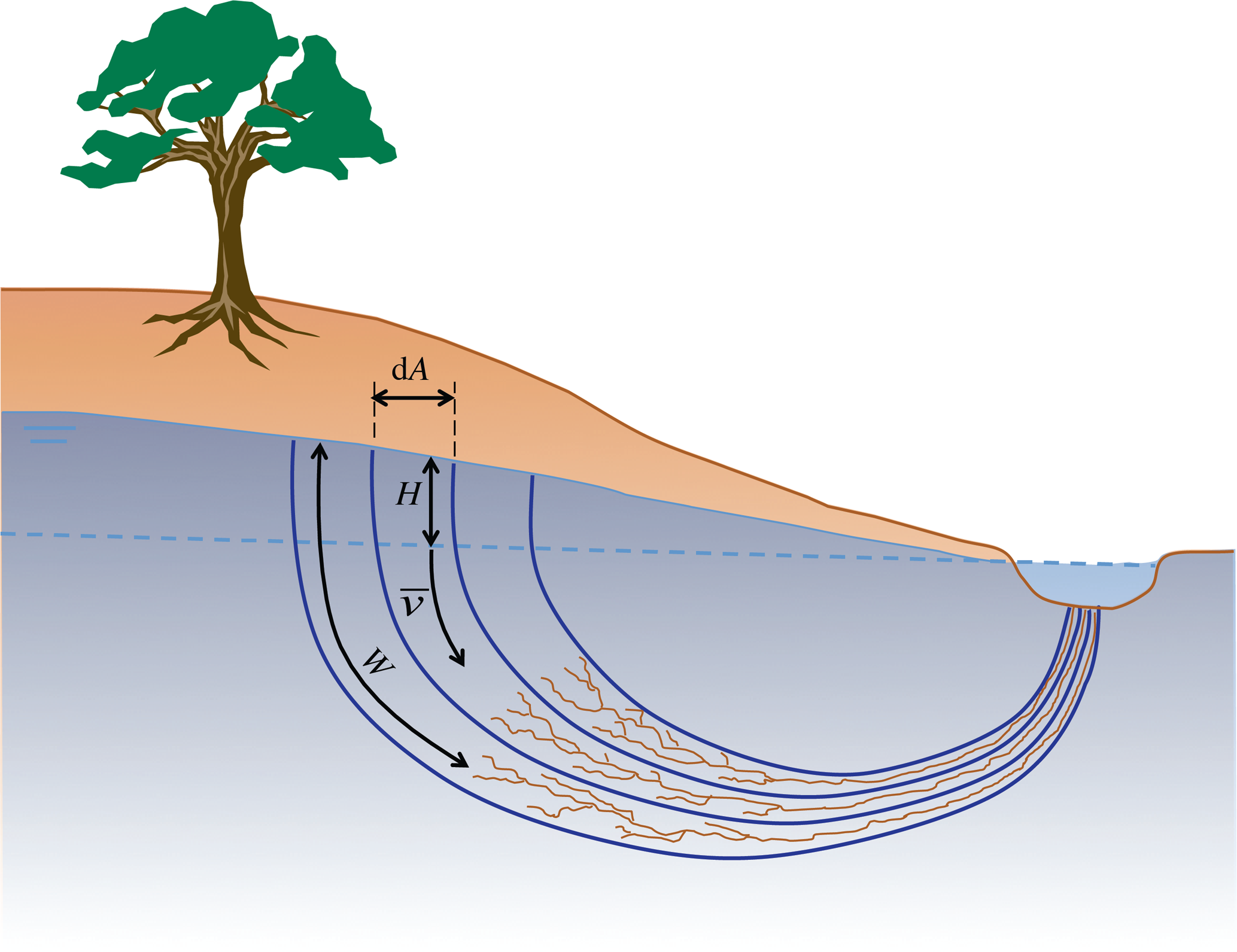
“Head-Dependent Flux” Boundaries (Cauchy)

Sometimes the amount of flux in or out of the system is depending ont he solution itself.

What it specifies: Relationship between flux and head difference

q_n = \frac{K_m}{M} \left[ h_m(x,y,z,t) - h(x,y,z,t) \right]

Parameters:

K_m = hydraulic conductivity of boundary layer
M = thickness of boundary layer
h_m = external head (e.g., river stage)

Key feature:

Flux depends on head difference — more realistic for many situations.

When to Use Cauchy Boundaries

Ideal for river-aquifer interactions:

River stage varies with time (h_m changes)
Riverbed acts as semi-permeable layer
Flow direction can reverse (gaining vs. losing stream)

Advantages:

More physically realistic
Automatically handles flow reversals
Accounts for resistance of boundary layer

Example:

During floods, h_m > h so water flows from river to aquifer. During droughts, h > h_m so aquifer feeds the river.

Choosing the Right Boundary Condition

Decision Matrix:

Dirichlet

Large water bodies
Known, stable water levels
Simple to implement

Neumann

Known recharge rates
Impermeable boundaries
Well pumping/injection

Cauchy

River-aquifer exchange
Variable external conditions
Semi-permeable boundaries

The choice depends on: physical setting, available data, and modeling objectives.

Initial Conditions: Starting Point for Transient Problems

For transient (time-dependent) problems, we need to specify where we start:

h(x, y, z, 0) = h_0(x, y, z)

What this means: At time zero, the hydraulic head at every point in the domain must be known.

Important:

Steady-state problems don’t need initial conditions — they find the equilibrium directly.

Why Initial Conditions Matter

Examples of initial conditions:

Aquifer at natural equilibrium before pumping
Known water table elevation from well measurements
Results from previous model run

Physical meaning: The system’s “starting configuration” before any changes occur.

Practical tip:

Often use steady-state solution as initial condition for transient problems.

Flow-net Analysis

Constructing the streamlines or the flowlines

Visualising Groundwater Flow

From Equations to Pictures

We can visualise the results using flow nets:

Two key components:

Streamlines (flow paths): show direction of water movement
Equipotential lines: contours of equal hydraulic head

Key property: In isotropic, homogeneous media, streamlines and equipotentials intersect at right angles.

Remember:

Water flows perpendicular to equipotential lines, from high head to low head.

Flowlines are our way of visualising the flow, without solving the flow equation.

The Mathematical Foundation

For 2D steady-state flow in isotropic, homogeneous media:

\frac{\partial^2 h}{\partial x^2} + \frac{\partial^2 h}{\partial y^2} = 0

This is Laplace’s equation - it has special mathematical properties that make flow nets possible.

Why 2D?

Many practical problems can be simplified to 2D, making flow nets a powerful tool.

Rules for Constructing Flow Nets

Geometric rules:

Orthogonality: Equipotentials ⊥ streamlines
Curvilinear squares: Lines form approximate squares
Equal spacing: Same head drop between equipotentials
Conservation: Same flow between adjacent streamlines

Boundary conditions:

No-flow boundaries → parallel to streamlines
Constant-head boundaries → parallel to equipotentials
Symmetry lines → can be treated as no-flow

The famous dam seepage problem

Flow net under dam — Seepage through permeable foundation

Practical tip:

Start with boundary conditions from page before, then sketch equipotentials and streamlines iteratively until squares form.

The famous dam seepage problem

Classic problem: seepage under a dam

Boundary conditions:

Left side: Constant head (upstream pool level)
Right side: Constant head (downstream pool level)
Bottom: No-flow boundary (impermeable bedrock)
Top: Free surface or no-flow

Result: Curved flow paths that form approximate squares

Reading the Flow Net

What the flow net tells us:

Flow direction: Follow the streamlines
Head distribution: Read from equipotential values
Flow concentration: Closer streamlines = higher velocity
Seepage quantity: Can be calculated from the net

Engineering applications:

Assess dam safety (uplift pressure)
Design drainage systems
Estimate seepage losses

Key insight:

Maximum head gradient (steepest flow) occurs where equipotentials are closest together.

Quantifying flow

Let’s consider the 1 dimensional example

For a single flow channel between two streamlines: consider the 1d Darcy equation Q = A q = -A K \frac{\partial h}{\partial x}

\Delta Q = T \Delta h \frac{\Delta W}{\Delta L}

Where:

\Delta Q = flow through one channel
T = transmissivity
\Delta h = head drop between equipotentials
\Delta W / \Delta L = width/length ratio (≈ 1 for squares)

Homogeneous aquifer — Streamlines and equipotentials under homogenous and isotropic conditions, flow is due to the constant heads applied at the left and right sides of the domain.

Another way of looking at it

Let’s say there are a total number of n_f flow channels and n_d equipotential drops.

\Delta Q = \frac{n_f}{n_d} T \Delta h

then the flow rate is equal to n_f \Delta Q and pressure drop is equal to n_d \Delta h.

Where:

\Delta Q = flow through one channel
T = transmissivity
\Delta h = head drop between equipotentials
\Delta W / \Delta L = width/length ratio (≈ 1 for squares)

Total Flow Calculation

For the entire flow system:

Q_{total} = \frac{n_f}{n_d} T \Delta H

Where:

n_f = number of flow channels (between streamlines)
n_d = number of equipotential drops
\Delta H = total head difference across system

Practical steps:

Count flow channels
Count equipotential intervals
Measure total head drop
Apply formula

What we learned

We explored the theoretical foundations of groundwater flow, covering:

Mathematical Framework: recognizing differential equations and their characteristics (dimensionality, steady-state vs transient)
Equation Derivation: conservation of mass in a representative elementary volume leading to the groundwater flow equation
Darcy’s Law Integration: combining flow relationships with conservation principles
Specialized Cases: steady-state flow, isotropic media (Laplace’s equation), and unconfined aquifers (Boussinesq equation)
Boundary Conditions: Dirichlet (specified head), Neumann (specified flux), and Cauchy (head-dependent flux) boundaries
Initial Conditions: starting points for transient problems and their physical significance
Flow Net Analysis: visual representation of flow patterns using streamlines and equipotentials
Practical Applications: dam seepage, flow quantification, and engineering design using flow nets